graph TD
S --> NP
S --> VP
NP --> I
VP --> VP1["VP"]
VP --> PP
VP1 --> V
VP1 --> NP1["NP"]
V --> ate
NP1 --> Det
NP1 --> N
Det --> my
N --> food
PP --> P
PP --> NP2["NP"]
P --> on
NP2 --> Det1["Det"]
Det1 --> the
NP2 --> N2["N"]
N2 --> table
Introuction
Imagine an 8 year old saying “I have infinite aura!”
And their friend replies “Oh yeah? Well I have infinity plus one aura!”
One of the parents says, “You can’t do that! Infinity is not a number!”
I bet you’ve probably seen something like this before. It does beg the question though - how big is infinity? Well, infinite, right? But you might have heard people say “some infinities are bigger than others”.
Hearing this from TikTok, people wrongly apply it to everything. They might say, “there are twice as many positive integers overall as there are even positive integers”, or “the number of nonnegative integers is one more than the number of positive integers”, or “there are wayyyy more complex numbers than real numbers”. This sounds about right, but it’s actually not.
Cardinality
To understand why these seemingly intuitive claims are actually wrong, we first need to make a very obvious distinction with numbers - cardinality vs ordinality. Ordinality is the position of a number. Infinity is ordinal if you take a limit as x approaches infinity of something. Cardinality is the number of elements in a set (a collection of distinguished objects where order doesn’t matter). Languages distinguish this naturally - “third place” means the person who got that award was behind two people in a race, while “three dogs” means we’re counting a set of dogs with three elements. When we talk about sizes as in number of elements, that’s cardinality.
Bijections
There can also be mappings between two sets. A one-to-one correspondence, or bijective function (bijection), is a mapping that is both injective and surjective. Injectivity means no two elements in the first set map to the same element in the second set. Surjectivity means every element in the second set is mapped to by at least one element in the first set.
A function being injective guarantees that the first set has at most the same cardinality as the second. If the first set had more elements, then from the pigeonhole principle, at least two elements of the first set would map to the same element of the second set.
A function being surjective guarantees that the first has at least the same cardinality.
This means if a function is both injective and surjective, the two sets have the same cardinality. So, if you can find a bijective function mapping the two sets, their sizes are equal.
Finite Examples
There are some trivial examples of bijections, such as Morse Code - each letter of the alphabet is mapped to a unique sequence of dots and dashes. Make sure to have pauses when the code is being expressed though, otherwise there may be multiple parses, and then it won’t be bijective. Another example is the IPA for phonemic transcription, as each phoneme (an abstract mental category - learn about it in my phonology blog post) is mapped to exactly one unique glyph.
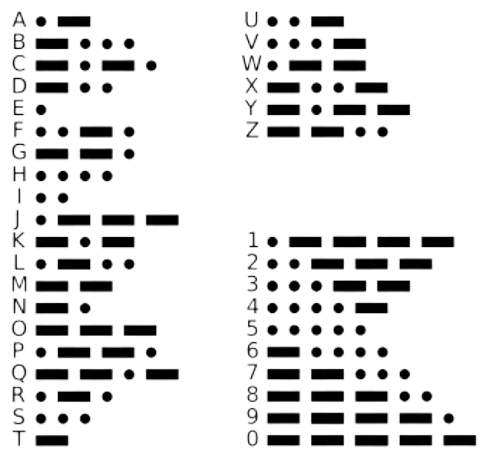
The thing about Morse Code, if it’s not immediately obvious, is that it’s only bijective if you actually keep divisions between each character’s encoding. Otherwise, two dots and one dash could either be “u” or “it” or “eet”.
There are some less trivial examples, too, with lots of applications in math problems. Consider starting at the point \((0, 0, 0)\), and you want to end at the point \((x, y, z)\), for \(x, y, z \in \mathbb{N}\), where you can only take one step up, front, and right each move. Then the number of paths, assuming no other constraints, would be \(\frac{(x+y+z)!}{x!y!z!}\). But this is the same as the number of rearrangements of a word with \(x\) instances of “\(A\)”, \(y\) instances of “\(B\)”, and \(z\) instances of “\(C\)”. Turns out, if we record each step, writing \(A\) for a move right, \(B\) for a move front, and \(C\) for a move up, it’s the exact same problem! And that encoding we just did was a bijective one.
These are all finite sets with the same size. Now is the moment we’re waiting for - seeing which infinities are actually bigger than other infinities.
Countable Infinity
Even though infinity is not a number, we can still give the symbol \(\aleph_0\) to represent the number of positive integers. This is also called countable infinity, because you could in theory count “\(1, 2, 3, \dots\)” forever if you were immortal.
The number of nonnegative integers is also \(\aleph_0\). The trick is to not see the set as just the positive integers with a \(0\) tacked on at the end. Instead, we start at \(0\), and go, “\(0, 1, 2, 3, \dots\)” forever. A bijective function that can map these two sets is \(f(x) = x-1\).
| \(1\) | \(2\) | \(3\) | \(\dots\) | \(x\) |
|---|---|---|---|---|
| \(0\) | \(1\) | \(2\) | \(\dots\) | \(x-1\) |
But how in the world can the number of even positive integers be the same as the number of positive integers overall? If you list “\(1, 2, 3, 4, 5, 6, \dots\)” and “\(2, 4, 6, \dots\)”, you’re not just removing one number but infinitely many numbers! However, try doubling all the positive integers and you’ll get the set of even positive integers, and \(f(x) = 2x\) is bijective! You can just count it forever like normal.
| \(1\) | \(2\) | \(3\) | \(\dots\) | \(x\) |
|---|---|---|---|---|
| \(2\) | \(4\) | \(6\) | \(\dots\) | \(2x\) |
The number of integers is the same as the number of positive integers. Now’s a good time to make it clear that a set’s cardinality is \(\aleph_0\) if you can index each element without missing or repeating anything - the bijection is between the object and the index. In this case, we can list out, “\(0, 1, -1, 2, -2, \dots\)” and everything will be accounted for - no need to put infinitely more numbers before the set of nonnegative integers.
| \(1\) | \(2\) | \(3\) | \(4\) | \(5\) | \(\dots\) |
|---|---|---|---|---|---|
| \(0\) | \(1\) | \(-1\) | \(2\) | \(-2\) | \(\dots\) |
We can also list out the rational numbers.
Basically, we first write the rational numbers in a grid, where the numerator and denominator are both positive integers (yes, technically rational numbers include negative numbers too, but once we show that we can list out the rational numbers, we can then use the same alternating technique shown in the previous example to account for negative numbers).
| \(\frac{1}{1}\) | \(\frac{1}{2}\) | \(\frac{1}{3}\) | \(\frac{1}{4}\) | \(\dots\) |
|---|---|---|---|---|
| \(\frac{2}{1}\) | \(\frac{2}{2}\) | \(\frac{2}{3}\) | \(\frac{2}{4}\) | \(\dots\) |
| \(\frac{3}{1}\) | \(\frac{3}{2}\) | \(\frac{3}{3}\) | \(\frac{3}{4}\) | \(\dots\) |
| \(\vdots\) | \(\vdots\) | \(\vdots\) | \(\vdots\) | \(\ddots\) |
Then we can zig-zag through the grid. So, we’d go \(\frac{1}{1}, \frac{2, 1}, \frac{1}{2}, \frac{1}{3}, \frac{2}{2}\), and so on. However, did you notice what went wrong? We repeated some numbers, as \(\frac{1}{1}\) is the same as \(\frac{2}{2}\). The fix is simple. Just skip them! And it’s perfectly valid too - we still end up being able to list out every rational number. So instead of going from \(\frac{1}{3}\) to \(\frac{2}{2}\), we go straight to \(\frac{3}{1}\). Thus, the rationals are countable.
Uncountable Infinity
It only makes sense that reals would also be countable… right? However, Cantor showed that this leads to a contradiction. (Show here)
Suppose you could actually list out every real number between 0 and 1. Then it might look like this:
| \(\mathbf{1.}\) | \(0.\) | \(1\) | \(6\) | \(2\) | \(\dots\) |
| \(\mathbf{2.}\) | \(0.\) | \(7\) | \(1\) | \(8\) | \(\dots\) |
| \(\mathbf{3.}\) | \(0.\) | \(3\) | \(1\) | \(5\) | \(\dots\) |
| \(\vdots\) | \(\vdots\) | \(\vdots\) | \(\vdots\) | \(\vdots\) | \(\ddots\) |
Looks fine, right? We can just put another random real number between \(0\) and \(1\) each time! But look what happens now if we construct a new number.
The first digit will be one more than the first digit of the first number, the second digit will be one more than the second digit of the second number, and so on. (It doesn’t actually matter if it’s actually one more, as long as they’re all different; for the purposes of this example, the convention is that \(9\) goes to \(0\)). So, using the table above, it would look like \(0.226\dots\). It’s not in the list, because it differs from the first number, and the second, and the third, and so on, by at least one digit! Since this is a contradiction, it must be that the real numbers are uncountable, with a greater cardinality than the \(\aleph_0\), because even if you list them out, not all of them will fit. We call this uncountable infinity.
Cardinality of Uncountable Infinity
A bit more research would tell you that the cardinality of the reals is \(2^{\aleph_0}\). When I first learned this, I immediately thought of the number of subsets of integers. Remember that for finite sets of cardinality \(n\), the number of subsets is \(2^n\).
Proof of the \(2^n\) thing, if you didn’t know already
There’s a few ways to think of this. The most straightforward is to go through each element in the set. It’s either in the subset, or it’s not, so there’s two choices. Each element’s choice is independent of the others. Hence the total number of \(2^n\).
Another way is to think of it is to do casework on the size of the subset. For a subset of size \(0\), there’s \(\binom{n}{0}\) ways to do this. For \(1\), it’s \(\binom{n}{1}\). For \(67\), provided that \(n \geq 67\), it’s \(\binom{n}{67}\). Adding all the cases, we get \(\sum\limits_{k=0}^n \binom{n}{k}\). This looks a lot like the binomial theorem, where \((a+b)^n = \sum\limits_{k=0}^n a^k b^{n-k} \binom{n}{k}\). In this case, \(a = b = 1\), so it’s \((1+1)^n = 2^n\).
Yet another way is to use induction. For the base case of \(n=1\), there’s two options - the element is in the subset, or not. Assuming the number of subsets of a set of size \(k\) is \(2^k\), we can look at \(k+1\) now. Either the \(k+1\) th element is in the subset, or it isn’t. So, for each of the \(2^k\) subsets, this doubles from the two cases, yielding \(2^{k+1}\). Yay, induction did its inductioning!
There’s a gazillion other ways to prove this, but fall into that rabbit hole in your own time.
Well, alright. First, let’s convert every real number from base \(10\) to binary. We know it must be bijective, because ultimately, both are just symbolic representations of the same thing, which is a point in space between \(0\) and \(1\). Yeah, that’s very unrigorous, but we can just assume it’s been proven before, because that’s not the point.
So every real number between \(0\) and \(1\) can just be represented as a sequence of \(0\)’s and \(1\)’s, preceded by a \(0\) and a decimal point. However, since all the real numbers have the same \(0\) and a decimal point, we can just ignore that, as another bijective operation would be to get rid of that.
A bijective encoding of this sequence would be to index it. \(0, 1, 1, 0, 1, 1, \dots\) could be encoded as \(2, 3, 5, 6, \dots\), because including an index means its corresponding digit is a \(1\), while omitting it means it’s a \(0\). Digit \(1\) is \(0\), digit \(2\) is \(1\), and so on. Since the meaning can be uniquely recovered both ways, it’s a bijection.
Note that what we have is quite literally just a subset of integers. Because of stacking a bunch of bijective operations, we have a single bijection between the set of reals between \(0\) and \(1\) and the set of subsets of integers. The number of integers is \(\aleph_0\), so the number of subsets of integers is \(2^{\aleph_0}\), so the number of reals between \(0\) and \(1\) is this too.
Other uncountable infinities
But now we need to show that the number of reals between \(0\) and \(1\) is the same as the number of reals overall. First, note that \(f(x) = \pi x - \frac{\pi}{2}\) is a bijection, because it’s just linear. This gets us the set of real numbers from \(-\frac{\pi}{2}\) to \(\frac{\pi}{2}\). Then, we use \(g(x) = \tan(x)\) to map this to the set of all real numbers, because \(\tan(x)\) is bijective for \(-\frac{\pi}{2} < x < \frac{\pi}{2}\). In my opinion, these is the cleanest one, but there’s others you can do.
If you thought we’re done, not quite yet. We still need to show that the complex numbers have a cardinality of \(2^{\aleph_0}\) too. First of all, since any complex number \(z\) can be written as \(a+bi\) for \(a, b \in \mathbb{R}\), this can be represented as an ordered pair of real numbers \((a, b)\). Since there are \(2^{\aleph_0}\) possibilies for \(a\) and \(b\) each, we multiply them to find the number of possibilities for \((a, b)\), so that yields \(2^{\aleph_0 + \aleph_0}\). We know for sure that \(\aleph_0 + \aleph_0 = \aleph_0\). This is because, for example, the number of integers is \(\aleph_0\). So are the number of even and odd integers. To find the total number of integers, since odd and even integers are disjoint, we simply add their cardinalities, so we get \(\aleph_0 + \aleph_0 = \aleph_0\), so \(|\mathbb{C}| = 2^{\aleph_0} = |\mathbb{R}|\).
Conclusion
So now you are an expert on the intuition behind how we measure infinity! Since I’m almost finished with my linguistics articles, I’ll be shifting more towards math.
Further Information
This is the original proof by Cantor. It’s based on infinite sequences rather than decimals, but basically the same idea.
This is a Quanta article about Cantor, going over both the math itself and the historical context.
For the finite examples, I showed the pathwalking as word rearrangement trick. There are some other finite bijections that are very cool. One that I personally like is how a syntax tree can be encoded as brackets, and this encoding is bijective because you can recover the same information both ways. For example, both of these encode the same internal structure and labels of of “I ate my food on the table”, but I think you can take a wild guess on which one people prefer.
S[NP[“I”]VP[VP[V[“ate”]NP[Det[“my”]N[“food”]]]PP[P[“on”]NP[Det[“the”]N[“table”]]]]]